Large scale analysis of mobility data and language during the COVID19 pandemic
Predicting the Spread of COVID-19 based on Mobility Data
Paper: https://arxiv.org/pdf/2009.08388.pdf
Code & Data: https://github.com/geopanag/pandemic_tgnn
Introduction
During a pandemic, accurately predicting the spread of the infection is of paramount importance to governments and policymakers in order to impose measures to combat the spread of the virus or decide on the allocation of healthcare resources. One of the main objectives of the project is to study the impact of population mobility on the spread of COVID-19. Furthermore, an interesting research direction is to investigate whether by giving predictive models access to population mobility data, we can achieve more accurate predictions of the number of COVID-19 cases.
Given the severity of the pandemic and the need for accurate forecasting of the disease spread, machine learning, and artificial intelligence approaches have emerged as a promising methodology to combat COVID-19. To predict the spread of COVID-19, ideally, we would like to have access to the social network of all individuals and to make predictions based on the interactions between them. However, in the absence of such data, we consider an alternative problem: predicting the development of the disease based on mass mobility data, i.e., how many people moved from one place to another. Mobility inside a region can be regarded as a proxy of the interaction i.e., the more people move, the higher the risk of transmission inside the region. Interestingly, mobility between different regions is known to play a crucial role in the growth of the pandemic, especially for long range travels [Colizza et al., 2006; Soriano-Panos et al., 2020]. Mobility gives rise to a natural graph representation allowing the application of recent relational learning techniques such as graph neural networks (GNNs).
GNNs have been applied to a wide variety of tasks, including node classification [Kipf and Welling, 2017], graph classification [Morris et al., 2019], text categorization [Nikolentzos et al., 2020] and recommendation [Ying et al., 2018]. GNNs capitalize on the concept of message passing, that is, at every iteration, the representation of each vertex is updated based on messages received from its neighbors. Since GNNs have been successfully applied to several real-world problems, we now investigate their effectiveness in forecasting COVID-19. We have focused on the problem of predicting the number of confirmed COVID-19 cases in each region of a country. Our model captures both spatial and temporal information, thus combining mobility data with the history of COVID-19 cases. Furthermore, since the availability of data is limited at the start of the outbreak in a country, we have employed a transfer learning method based on Model-Agnostic Meta-Learning to capitalize on knowledge from other countries’ models.
Data
Facebook has released several datasets in the scope of the Data For Good program to help researchers better understand the dynamics of the COVID-19 and forecast the spread of the disease. In our study, we used a dataset that consists of measures of human mobility between administrative NUTS3 regions. The data is collected directly from mobile phones that have the Facebook application installed and the Location History setting enabled. The raw data contains three recordings per day (i.e., midnight, morning, and afternoon), indicating the number of people moving from one region to another at that point of the day. We computed a single value for each day and each pair of regions by aggregating these three values. We focused on 4 European countries: France, Italy, Spain, and England. The number of cases in the different regions of the 4 considered countries was collected from open data listed in the following github repository: https://github.com/geopanag/pandemic_tgnn along with the code and the aggregated mobility data. An overview of the preprocessed data can be found in the following Table.
| Country | Time | Regions | Avg new cases |
|---|---|---|---|
| France | 10/3-12/5 | 81 | 7.5 |
| Italy | 24/2-12/5 | 105 | 25.65 |
| England | 13/3-12/5 | 129 | 16.7 |
| Spain | 12/3-12/5 | 35 | 61 |
The start date is the earliest date for which we have both mobility data and data related to the number of cases available. Some regions were removed either because they did not have any COVID-19 cases or because they could not be mapped to the Facebook mobility data.
Methodology
We first need to mention that our analysis involves a series of assumptions. First, we assumed that people that use Facebook on their mobile phones with Location History enabled constitute a uniform random sample of the general population. Second, we assumed that the number of cases in a region reported by the authorities is a representative sample of the number of people that have been actually infected by the virus. Finally, we hypothesize that the more people move from one region to another or within a region, the higher the probability that people in the receiving region are infected by the virus. This is a well-known observation in the field of epidemics [Colizza et al., 2006; Soriano-Panos et al., 2020], and motivates the use of a message passing procedure as we delineate below.
Graph Construction. We chose to represent each country as a graph G=(V,E) where n=|V| denotes the number of nodes. Specifically, given a country, we create a series of graphs, each corresponding to a specific date t, i.e., G(t),…, G(T). Let A(t),…,A(T) denote the adjacency matrices of these graphs. A single date’s mobility data is transformed into a weighted, directed graph whose vertices represent the NUTS3 regions and edges capture the mobility patterns. For instance, the weight of the edge between nodes v and u in graph G(t) denotes the total number of people that moved from region v to region u at time t. Note that these graphs can also contain self-loops which correspond to the mobility behavior within the regions. The mobility between administrative regions u and v at time t forms an edge which, multiplied by the number of cases c(t)(u) of region u at time t, provides a relative score expressing how many infected individuals might have moved from u to v. To be more specific, let x(t)(u) = (c(t-d)(u),…, c(t)(u)) be a vector of node attributes, which contains the number of cases for each one of the past d days in region u. We use the cases of multiple days instead of just the day before the prediction because case reporting is highly irregular between days, especially in decentralized regions. Intuitively, message passing over this network computes a feature vector for each region with a combined score from all regions, as illustrated below.
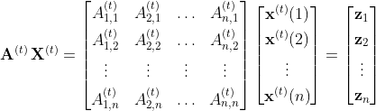
where X(t) is a matrix whose rows contain the attributes of the different regions. In this case, zu is a vector that combines the mobility within and towards region u with the number of reported cases both in u and in all the other regions. Here, we would like to stress the importance of the mobility patterns within a region u which correspond to good indicators of the evolution of the disease, especially during lockdown periods.
Models. To model the dynamics of the spreading process, we used two instances of a well-known family of GNNs, known as message passing neural networks (MPNNs) [Gilmer et al., 2017]. These networks consist of a series of neighborhood aggregation layers. Each layer uses the graph structure and the node feature vectors from the previous layer to generate new representations for the nodes. Specifically, we employed the following 3 models:
-
MPNN: To update the representations of the vertices of each of the input graphs, this model uses the following neighborhood aggregation scheme:
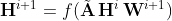
where Hi is a matrix that contains the node representations of the previous layer, with H0 = X, Wi is the matrix of trainable parameters of layer i, and f is a non-linear activation function such as ReLU. We also normalized the adjacency matrix A such that the sum of the weights of the incoming edges of each node is equal to 1. Note that for simplicity of notation, we have omitted the time index. The above model is in fact applied to all the input graphs G(1),…, G(T) separately. Given a model with K neighborhood aggregation layers, the matrices A and H0,…, HK are specific to a single graph, while the weight matrices W1,…, WK are shared across all graphs. Typically, an MPNN contains K neighborhood aggregation layers. As the number of neighborhood aggregation layers increases, the final node features capture more and more global information. However, retaining local, intermediary information might be useful as well. Thus, we concatenated the matrices H0, H1,…, HK horizontally, i.e., H = CONCAT(H0, H1,…, HK) and the rows of the emerging matrix Η can be regarded as vertex representations that encode multi-scale structural information, including the initial features of the node. In other words, we utilized skip connections from each layer to the output layer which consists of a sequence of fully-connected layers. Note that we applied the ReLU function to the output of the network since the number of new cases is a nonnegative integer. We chose the mean squared error as our loss function as shown below:
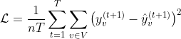
This function compares the reported number of cases for region v at day t+1 against the predicted number of cases for that region. An overview of the MPNN is shown in the following Figure.
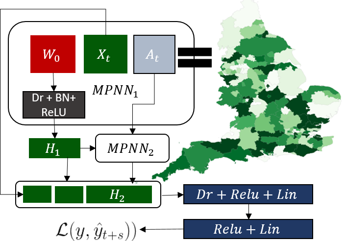
Overview of the proposed MPNN architecture -
MPNN+LSTM In order to take advantage of the temporal correlation between the target and the confirmed cases in the past, we built a time-series version of our model using the different snapshots of the mobility graph. Given a sequence of graphs G(0), G(1),…, G(T) that correspond to a sequence of dates, we utilized an MPNN at each time step, to obtain a sequence of representations H0, H1,…, HT. These representations were then fed into a Long-Short Term Memory network (LSTM) [Graves and Jaitly, 2014] which can capture the long-range temporal dependencies in time series. We expect the hidden states of an LSTM to capture the spreading dynamics based on the mobility information encoded into the node representations. We used a stack of two LSTM layers. The new representations of the regions correspond to the hidden state of the last time step of the second LSTM layer. These representations were then passed on to an output layer similar to the MPNN, along with the initial features for each time step. Note that this model resembles other attempts to spatio-temporal prediction, but instead of convolutional [Yao et al., 2018], it employs message passing layers. The MPNN+LSTM model is illustrated in the following Figure.
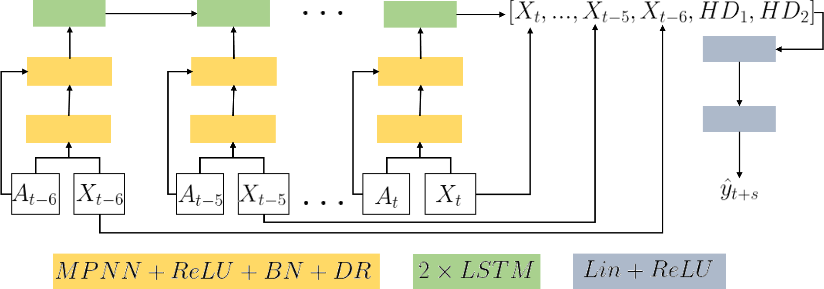
Overview of the MPNN LSTM architecture -
MPNN+TL Note that the different countries were hit by the pandemic at different times. Indeed, there are cases where once the epidemic starts developing in one country, it has already stabilized in another. Furthermore, a new wave of COVID-19 is very likely to share fundamental characteristics with the previous ones, as it is the same virus. This additional information may prove rather important in case of insufficient training data. In our setting, as discussed later on, the model starts predicting as early as the 15th day of the dataset. In such a scenario, the model has access to a few samples to learn from (split into validation and training sets), while it is used to make predictions for as far as 14 days ahead. Given the inherent need for data in neural networks, this setting is rather challenging. Moreover, our intuition is that a model trained in the whole cycle or an advanced stage of the epidemic can capture patterns of its different phases, which is missing from a new model working in a country at the start of its infection. To incorporate past knowledge from models running in other countries, we separated our data into tasks and developed an adaptation of Model-Agnostic Meta-Learning (MAML) [Finn et al., 2017]. Thus, given a specific country, our model was trained on data from other countries and evaluated on that country.
Results & Discussion
Experimental Setup. In our experiments, we trained the models using data from day 1 to day T, and then used the model to predict the number of cases for each one of the next dt days (i.e., from day T+1 to day T+dt). Our goal was to evaluate the effectiveness of the model in short-, mid- and long-term predictions. Therefore, we set dt equal to 14. We expect the short-term predictions (i.e., small values of dt) to be more accurate than the long-term predictions (i.e., large values of dt). Note that we trained a different model to predict the number of cases for days T+i and T+j where i,j > 0 and i <= j. Therefore, each model focuses on predicting the number of cases after a fixed time horizon, ranging from 1 day to 14 days. With regards to the value of T, it was initially set equal to 14 and was gradually increased (one day at a time). Therefore, the size of the training set increases as time progresses. Note that a different model was trained for each value of T. Furthermore, for each value of T, to identify the best model, we built a validation set which contains the samples corresponding to days T-1, T-3, T-5, T-7 and T-9, such that the training and validation sets have no overlap with the test set.
With regards to the hyperparameters of the MPNN, we trained the models for a maximum of 500 epochs with early stopping after 50 epochs of patience. Early stopping starts to occur from the 100th epoch and onward. We set the batch size to 8. We used the Adam optimizer with a learning rate of 10-3. We used 2 neighborhood aggregation layers with ReLU activation functions. We set the number of hidden units of the neighborhood aggregation layers to 64. Batch normalization and dropout were applied to the output of every neighborhood aggregation layer, with a dropout ratio of 0.5. We stored the model that achieved the highest validation accuracy in the disk and then retrieved it to make predictions about the test samples. For the MPNN+LSTM model, the dimensionality of the hidden states of the LSTMs was set equal to 64. We evaluated the performance of a model by comparing the predicted total number of cases in each region versus the corresponding ground truth, throughout the test set:
We compared the proposed models against the following baselines and benchmark methods, which have been applied to the problem of COVID-19 forecasting:
- AVG: The average number of cases for the specific region up to the time of the test day.
- AVG_WINDOW: The average number of cases in the past d days for the specific region where d is the size of the window.
- LAST_DAY: The number of cases of the previous day is the prediction for the next days.
- LSTM [Chimmoula and Zhang, 2020]: A two-layer LSTM that takes as input the sequence of new cases in a region for the previous week. %It has been used for COVID-19 forecasting.
- ARIMA [Kufel, 2020]: A simple autoregressive moving average model where the input is the whole time-series of the region up to before the testing day.
- PROPHET [Mahmud, 2020]: A forecasting model for various types of time series: https://github.com/facebook/prophet. The input is similar to ARIMA.
- TL_BASE: An MPNN that is trained on all data from the three countries and the train set of the fourth (concatenated), and tested on the test set of the fourth. This serves as a baseline to quantify the usefulness of MPNN+TL.
We should note here that we cannot utilize models that work with recoveries and deaths such as SEIR because we only have the confirmed cases. That said, a simple approach is to run SI at every T with a β taken from the COVID-19 literature, along with the number of infected people at T and the population. In the preliminary experiments, however, this provided errors in a different scale than the ones mentioned here, which is why we have not experimented further.
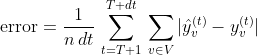
Results. The average error per region for each one of the next 14 days is illustrated in the following Figure.
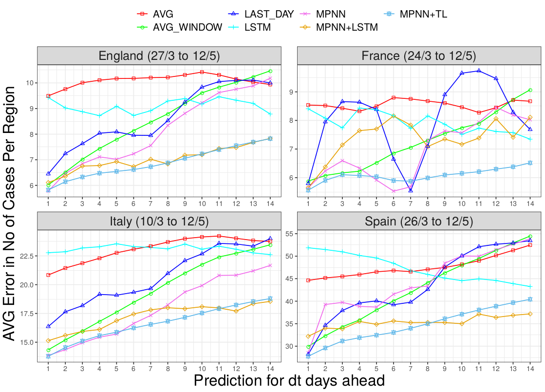
We observe that the proposed models yield lower average errors compared to the baselines, MPNN+TL having the best performance. In terms of short-term predictions its performance is close to some baselines, but the difference increases for longer scopes. Even simple baselines can be competitive at predicting the next day’s number of cases since proximal samples for the same region from the same phases of the pandemic tend to have a similar number of cases. However, a prediction that goes deeper in time requires the identification of more persistent patterns. In the case of our model, as mentioned above, we aim to capture unregistered cases moving from one region to the other or spreading the disease in their new region. These cases would inevitably take a few days to appear, due to the delay of symptoms associated with COVID-19. This is why MPNN performs well throughout the 14-days window. The results also demonstrate the benefit of transfer learning techniques since MPNN+TL outperforms MPNN and its baseline TL_BASE in all cases. We expect MPNN to perform similar towards the end of the dataset, when the training of both models has become similar due to the number of epochs and. The main difference occurs when T is small, where the training samples are scarce and MPNN is unable to capture the underlying dynamics. One way to see this is again the accuracy of MPNN+TL in the long-term predictions. Due to the size of the prediction window, long term tasks have diminished train set, meaning if the task is to predict t+14 and the set ends at day 60, t+14 training will stop at day 46 while the t+1 will stop at 59. Thus, MPNN performs similarly at the short-term predictions but fails compared to MPNN+TL in the long term.
Note that for clarity of illustration, we chose not to visualize the performance of PROPHET and ARIMA in the above Figure as their error was distorting the plot. However, we present in the Table below the average error for the predictions where dt takes three values: 3, 7 and 14.
Overall, it is clear that the time series methods (i.e., LSTM, PROPHET, and ARIMA) and the temporal variant of our method MPNN+LSTM yield quite inaccurate predictions. Apart from the inherent difficulty of learning with time-series data, which we analyze further below, this might also happen because of the nature of the epidemic curve. Specifically, sequential models, that are trained with values that tend to increase, are impossible to predict decreasing or stable values. For instance, in our dataset, once the models have enough samples to learn from, there is a transition in the phase of the epidemic due to lockdown measures. The same applies when the epidemic starts to recede at the start of May.
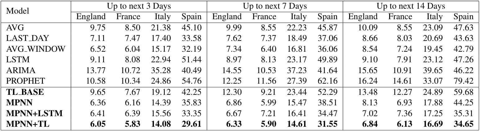
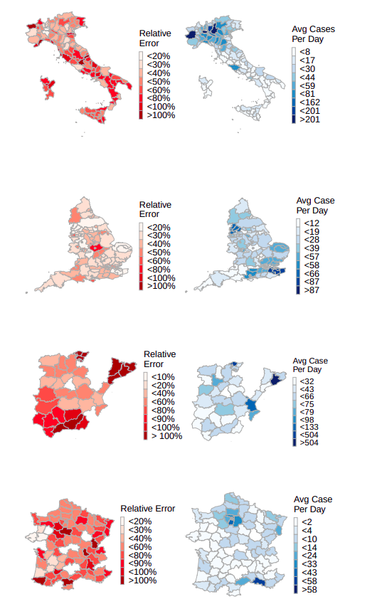
Our error function treats all regions equivalently, independent of the region-specific population and the number of cases, i.e., a region with 10 cases per day should not be treated the same as a region with 1000. We need a measure to take into account the region-specific characteristics as well as the time. Towards this end, we computed the deviation between the average predicted and the actual average number of cases over the next 5 days (not to be confused with the average error for the next x days in the above Table). The relative error of each region is defined as:
The relative error along with the average number of cases are illustrated in the Figures below.
 |
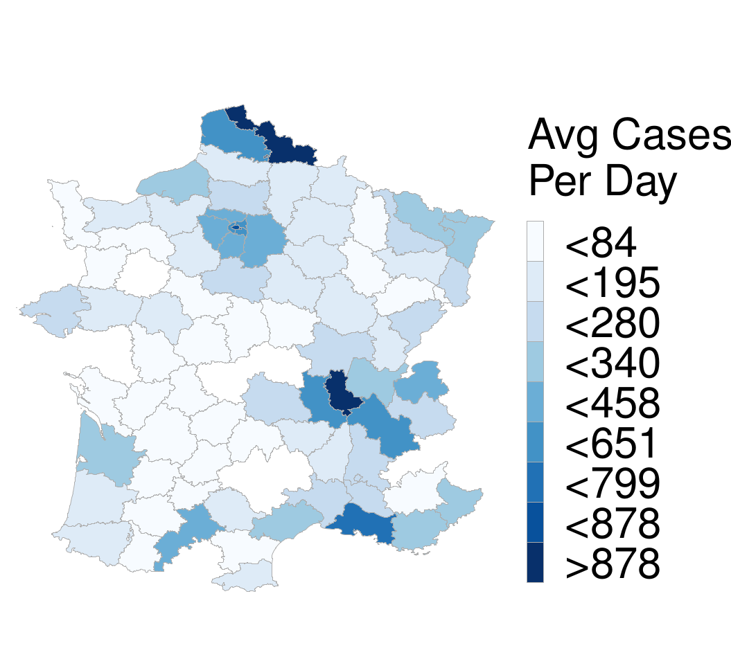 |
One can see that the regions with high relative error are the ones with the fewest cases. On the other hand, the regions with the highest number of cases tend to have much smaller relative error, less than 20% to be exact, with the exception of one region in Spain. This indicates that our model indeed produces accurate predictions that could be useful in resource allocation and policy-making during the pandemic.
he above Figure also allows us to evaluate the method more objectively. From a machine learning perspective, one may argue that even though the MPNN+TL outperforms the baselines, their predictions are not very accurate in terms of average error. This is partially explained due to the inherent problems of the dataset as well as the assumption that case reporting is standard throughout the regions. We expect a large improvement in performance in case a standard methodology for case reporting is adopted and the number of tests per region remains constant and proportional to the population. Having said that, utilizing such a model in practice is more than feasible as the difference in scale is more useful at the regional level. In other words, a region predicted to have 10 new cases in the next 5 days will generally have similar needs (e.g., hospital capacity needs) with a region with 5 or 15 real cases (50% error). On the other hand, predicting 500 instead of 1000 cases, although identical in terms of relative error, can prove disastrous. This is not the case for our model, since the regions with large relative error tend to have a small number of cases, e.g., the model may predict 20 cases instead of 10 (100% error), which is arguably not significant.
Further Experimental Results
We performed some additional experiments to predict the number of confirmed COVID-19 cases in the different regions of France for a longer period (from September 14 2020 to January 7 2021). The overall performance of the proposed model and the baselines is illustrated in the following Figure.
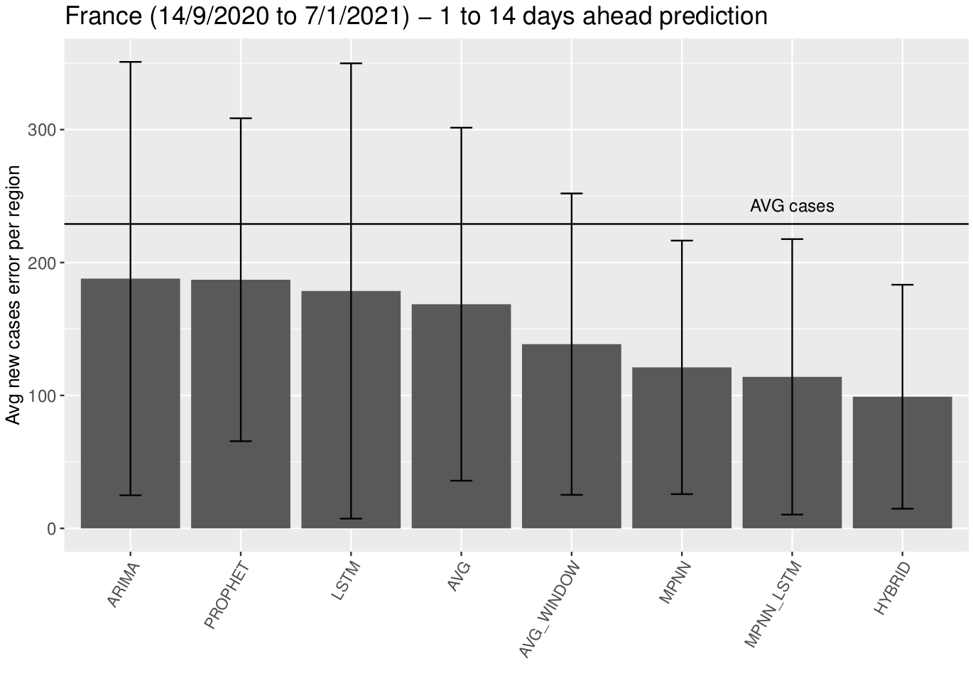
In the above Figure, HYBRID corresponds to a combination of the MPNN and MPNN+LSTM models. We can see that the proposed models outperform the baselines. In fact, the HYBRID approach is the best-performing method. We need to mention that the average error of all the approaches is quite large, and thus they all fail to make very accurate predictions. Even, the HYBRID approach yields an average error of approximately 100 cases per day. This is mainly related to the inconsistencies in case reporting. In the following Figure, we also show the average error per region for each one of the next 14 days.
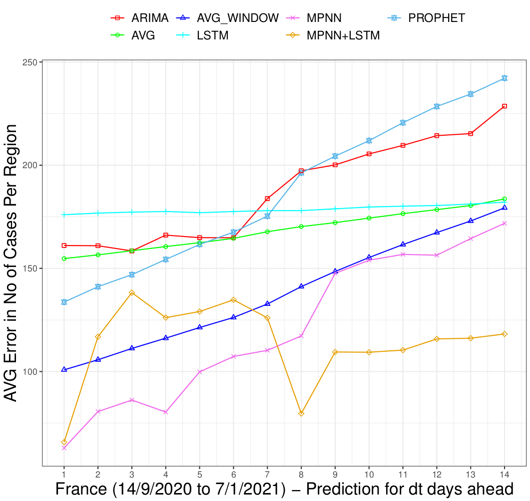
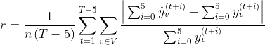
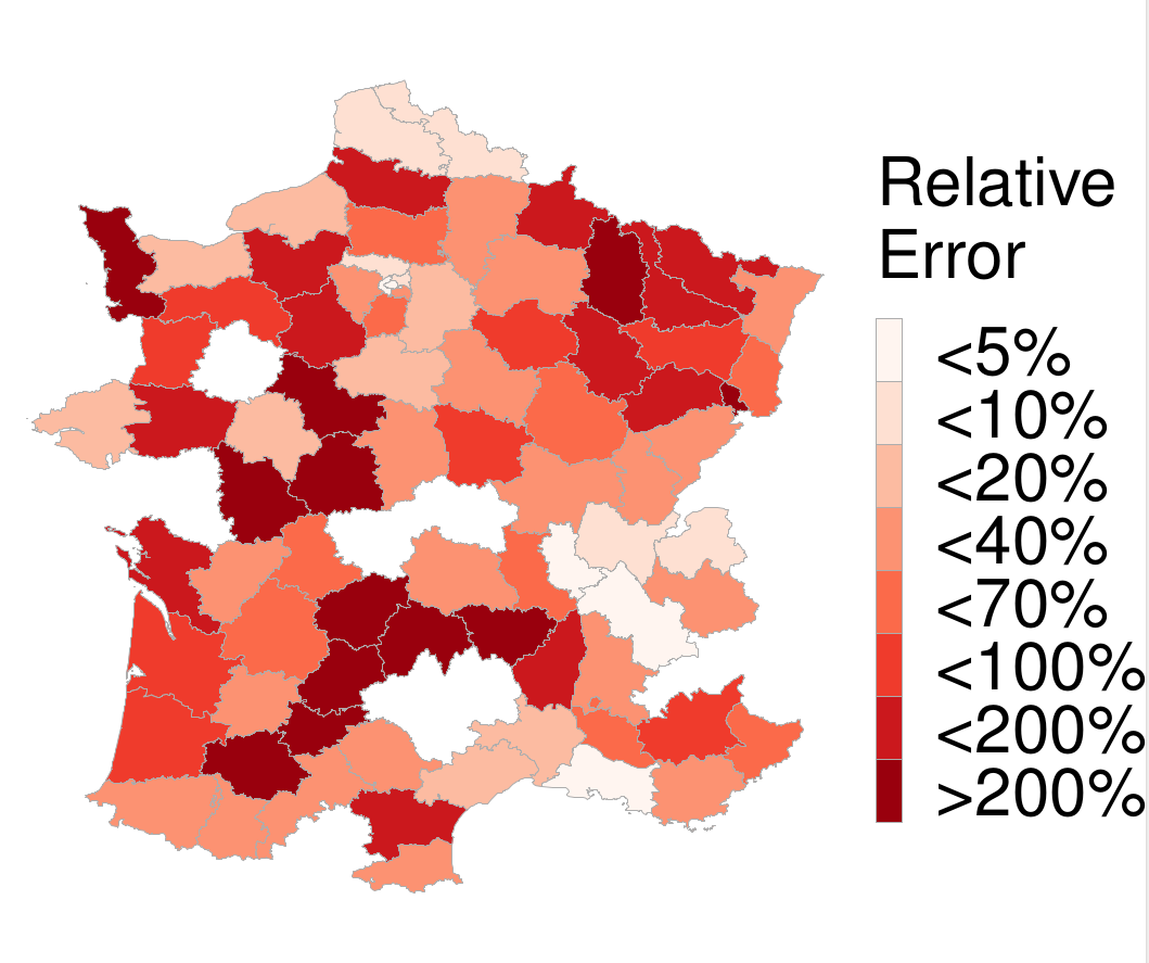
We can see that the proposed models outperform the baselines. Furthermore, the predictions of the MPNN model are relatively accurate in the first 4 days, while the MPNN+LSTM model outperforms all the other approaches in the case of long-term predictions (i.e., from day 8 and thereafter). Finally, the relative error along with the average number of cases in the different departments of France are illustrated in the Figures below.
|
|
|
We can see that the relative error is very low in departments whose population and average number of cases are very large (e.g., Île-de-France). This demonstrates that the model yields good performance in predicting the number of cases in regions of higher risk. On the other hand, the highest relative error occurs in departments whose population and number of cases are small, thus in regions where predicting the actual number of future cases is not of as high significance as in more densely populated territories.