Lemma 4. -- Let ![]() , ...,
, ..., ![]() ,
, ![]() be polynomials in
be polynomials in
![]() such that
such that
![]() and
and
![]() is a prime
differential ideal
is a prime
differential ideal ![]() of differential dimension
of differential dimension ![]() . Let
. Let
![]() ,
,
Then, the order of ![]() is equal to
is equal to ![]() if
if
![]() and strictly
lower than
and strictly
lower than ![]() if not.
if not.
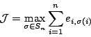
The integer ![]() is known as the Jacobi number and
is known as the Jacobi number and
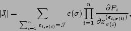
![]() is the
truncated jacobian (determinans mancum in
[7]). We denote by
is the
truncated jacobian (determinans mancum in
[7]). We denote by ![]() the minimal integers such that
there exists a diagonal sum
the minimal integers such that
there exists a diagonal sum
![]() and
for all
and
for all ![]()
![]() is maximal among all
is maximal among all
![]() (see [4,7]).
(see [4,7]).
Sketch of the proof of theorem 3. -- In order to prove the
theorem, we consider any algebraic extension ![]() and construct
it as the quotient field of a prime differential ideal given by a
characteristic set
and construct
it as the quotient field of a prime differential ideal given by a
characteristic set ![]() in
in
![]() . The
extension
. The
extension
![]() is described by a prime differential
ideal, whose characteristic set
is described by a prime differential
ideal, whose characteristic set ![]() admits a number of elements
equal to
admits a number of elements
equal to
![]() .
.
Let ![]() be a set of
be a set of ![]() equations such that
equations such that
![]() , where
, where
![]() . Such a set
. Such a set ![]() exists, e.g.
exists, e.g. ![]() satisfies the
hypotheses if we take
satisfies the
hypotheses if we take
![]() . We may chose
. We may chose ![]() ,
,
![]() and
and ![]() such that the bound
such that the bound ![]() of lemma 4
is minimal. Now, we reorder the equations by increasing
of lemma 4
is minimal. Now, we reorder the equations by increasing ![]() ,
and for equal
,
and for equal ![]() , we take first the equations in
, we take first the equations in ![]() . Let
. Let
![]() be the smallest integer such that the first
be the smallest integer such that the first ![]() rows of
rows of
![]() are
not of full rank. We will also assume that we have chosen
are
not of full rank. We will also assume that we have chosen ![]() ,
,
![]() and
and ![]() with minimal
with minimal ![]() among those with minimal
among those with minimal ![]() .
.
Assume
![]() . Then, as the extension is algebraic, the truncated
jacobian
. Then, as the extension is algebraic, the truncated
jacobian
![]() should be
should be ![]() ; if not, the order of the extension
would be
; if not, the order of the extension
would be ![]() . Now, if the truncated jacobian is
. Now, if the truncated jacobian is ![]() , we can
construct by algebraic elimination a new set
, we can
construct by algebraic elimination a new set ![]() or a new
extension
or a new
extension ![]() , associated with a new characteristic set
, associated with a new characteristic set ![]() with
a smaller
with
a smaller ![]() , or an equal
, or an equal ![]() and a smaller
and a smaller ![]() . This contradicts
minimality. So,
. This contradicts
minimality. So, ![]() and
and
![]() .
.
This implies that there are ![]() variables
variables ![]() appearing in
appearing in ![]() with order
with order ![]() such that
such that
![]() for
for
![]() . We may assume those variables to be
. We may assume those variables to be
![]() after a reordering. This shows that
after a reordering. This shows that
![]() is algebraic, and so that
is algebraic, and so that
![]() is flat. height .9ex width .8ex depth -.1ex
is flat. height .9ex width .8ex depth -.1ex
The proof is a constructive one. Provided that the extensions ![]() ,
,
![]() and
and ![]() are given by generators and relations, we are able,
using characteristic sets computations, to construct a representation
of
are given by generators and relations, we are able,
using characteristic sets computations, to construct a representation
of ![]() as a flat extension. We investigate the algorithmic aspects of
that theorem which reduce to a sequence of algebraic eliminations. If
the computation could be in the worst case as difficult as algebraic
elimination could be, we may very often in practice deduce some
linearizing output from the parametrization without any elimination.
as a flat extension. We investigate the algorithmic aspects of
that theorem which reduce to a sequence of algebraic eliminations. If
the computation could be in the worst case as difficult as algebraic
elimination could be, we may very often in practice deduce some
linearizing output from the parametrization without any elimination.
It should be noted that, if the flatness notion may be defined in a
geometrical setting using
![]() functions, the equations are
most of the time polynomial in practice, making the algebraic
definition, with its algorithmic potentialities, of special interest.
functions, the equations are
most of the time polynomial in practice, making the algebraic
definition, with its algorithmic potentialities, of special interest.