Car.mw
Maple worksheet. Study of a flat model of a car with
Intrinsic and Apparent Singularities.
Joint work with Yirmeyahu J. Kaminski, Jean Lévine, François Ollivier
| > |
 |
| > |
 |
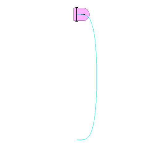
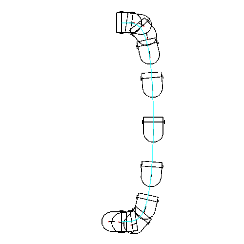
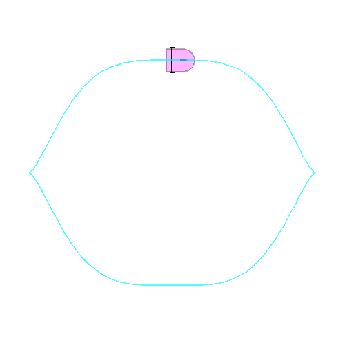
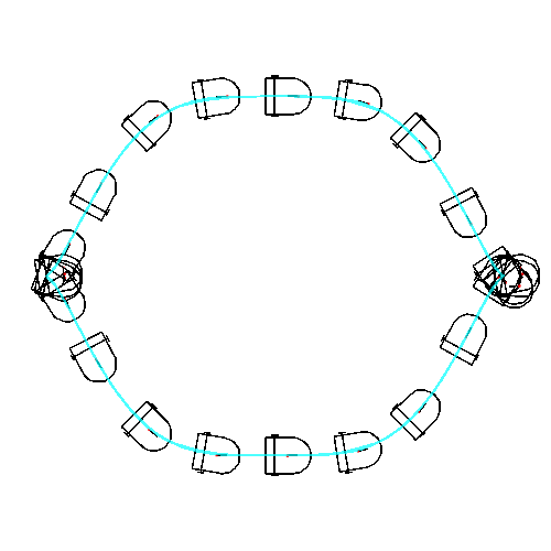
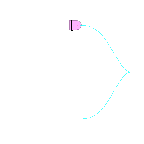
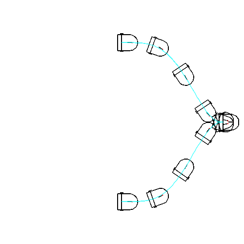
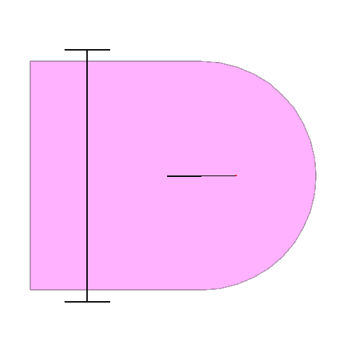
This function draws the car : x and y are the coordinates of the rear axle center, theta the angle of the car body and phi the angle of the front wheel. A red dot provides the orientation of this wheel.
If the global variable car_display is 0, the body of the car is a magenta polygon (used for animations). If not is just a black curve (used for superpositions).
| > |
 |
This functions computes the position of a car, described by the trajectory (f,g) of the middle of the rear axle. The functions f and g depend on the variable t and t0 that must be of type numeric, stands for the current time. The value of theta is stored using global variable theta_prev and theta is computed modulo Pi in order to minimize |theta_prev - theta|. The same thing is done for phi_prev.
| > |
 |
The trajectory is given by theta and psi= sin(theta)x-cos(theta)y. This may be seen as the limit of flat outputs given by a point of the rear axle, when the point goes to infinity. There is no more ambiguity about the value of theta, but theta_prev is stored together with phi_prev to allow combined use with rear_axle function.


| > |

 |
Parametrization of a trajectory. Functions x and y are used if 


Views is the list of times to be computed. N_size the size of the output picture. The global variable param_display controls the style of the output: an animation if param_output=0 a superposition of views if not.
| > |
 |
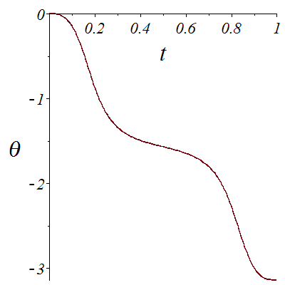
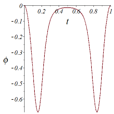
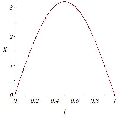
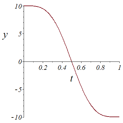
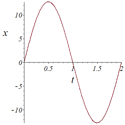
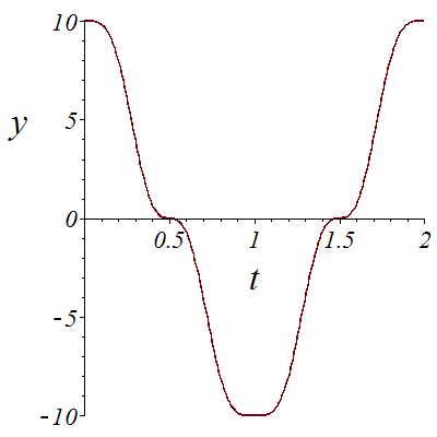
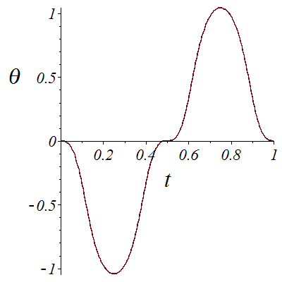
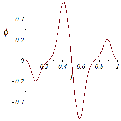
We denote the position of the car by the quintuple (x,y,theta,phi,u). Here the car goes from (0,10,0,0,10) at time t=0 to (0,-10,Pi,0,10) at time t=1.
| > |
![Y1 := `+`(`*`(A1, `*`(cos(`*`(Pi, `*`(t))))), `*`(B1, `*`(cos(`+`(`*`(3, `*`(Pi, `*`(t)))))))); -1; resu := solve([eval(Y1, t = 0) = 10, eval(diff(Y1, t, t), t = 0) = 0], [A1, B1]); -1; Y1 := subs(op(...](images/Car_62.gif)
![Y1 := `+`(`*`(A1, `*`(cos(`*`(Pi, `*`(t))))), `*`(B1, `*`(cos(`+`(`*`(3, `*`(Pi, `*`(t)))))))); -1; resu := solve([eval(Y1, t = 0) = 10, eval(diff(Y1, t, t), t = 0) = 0], [A1, B1]); -1; Y1 := subs(op(...](images/Car_63.gif) |
| > |
![Theta1_prev := 0.; -1; plot(theta1, 0 .. 1, font = [TIMES, ITALIC, 18], labelfont = [TIMES, ITALIC, 26], labels = [t, theta]); 1](images/Car_67.gif)
![Theta1_prev := 0.; -1; plot(theta1, 0 .. 1, font = [TIMES, ITALIC, 18], labelfont = [TIMES, ITALIC, 26], labels = [t, theta]); 1](images/Car_68.gif) |
| > |
![Phi1_prev := 0.; -1; plot(phi1, 0 .. 1, font = [TIMES, ITALIC, 18], labelfont = [TIMES, ITALIC, 26], labels = [t, phi])](images/Car_73.gif) |
| > |
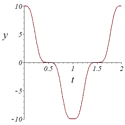
![plot(X1, t = 0 .. 1, font = [TIMES, ITALIC, 18], labelfont = [TIMES, ITALIC, 26], labels = [t, x]); 1; plot(Y1, t = 0 .. 1, font = [TIMES, ITALIC, 18], labelfont = [TIMES, ITALIC, 26], labels = [t, y]...](images/Car_75.gif)
![plot(X1, t = 0 .. 1, font = [TIMES, ITALIC, 18], labelfont = [TIMES, ITALIC, 26], labels = [t, x]); 1; plot(Y1, t = 0 .. 1, font = [TIMES, ITALIC, 18], labelfont = [TIMES, ITALIC, 26], labels = [t, y]...](images/Car_76.gif) |
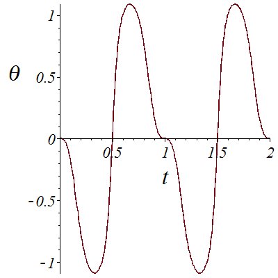
Here we want to go to from point (0,1,0,0,40) at t=0 to point (0,1,0,0,-40) at t=1, meaning that we start forward and arrive backward. For this, we need to cross a cusp where x~c_1-c_2*t^2, y~c3*t^3.
The presence of the cusp implies that diff(x,t) and diff(y,t) have a common factor that we need to remove to avoid trouble like: division by 0, or an extra loop in the curve, due to floating point inaccuracies, and the value of theta increase by Pi!
| > |
![Theta2_prev := 0; -1; plot(theta2, 0 .. 2, font = [TIMES, ITALIC, 18], labelfont = [TIMES, ITALIC, 26], labels = [t, theta]); 1](images/Car_96.gif)
![Theta2_prev := 0; -1; plot(theta2, 0 .. 2, font = [TIMES, ITALIC, 18], labelfont = [TIMES, ITALIC, 26], labels = [t, theta]); 1](images/Car_97.gif) |
| > |
![phi2(1.); -1; plot(phi2, 0 .. 2, font = [TIMES, ITALIC, 18], labelfont = [TIMES, ITALIC, 26], labels = [t, phi])](images/Car_102.gif) |
| > |
![plot(X2, t = 0 .. 2, font = [TIMES, ITALIC, 18], labelfont = [TIMES, ITALIC, 26], labels = [t, x]); 1; plot(Y2, t = 0 .. 2, font = [TIMES, ITALIC, 18], labelfont = [TIMES, ITALIC, 26], labels = [t, y]...](images/Car_104.gif)
![plot(X2, t = 0 .. 2, font = [TIMES, ITALIC, 18], labelfont = [TIMES, ITALIC, 26], labels = [t, x]); 1; plot(Y2, t = 0 .. 2, font = [TIMES, ITALIC, 18], labelfont = [TIMES, ITALIC, 26], labels = [t, y]...](images/Car_105.gif) |
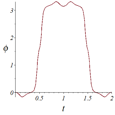
Like in the previous example, we want to go to from point (0,1,0,0,-40) at t=0 to point (0,1,0,0,-40) at t=1, meaning that we start forward and arrive backward. But this time, we want to have a better control on the value of phi and avoid it to reach Pi/2. For this, we need to cross a rhamphoid cusp with x~c_1-c_2*t^2, y~c3*t^5.
The presence of the rhamphoid cusp implies that diff(x,t) and diff(y,t) have a common factor that we need first to remove. But this is not enough, as we will have at this point x'=y'=theta'=0.
| > |
![Theta3_prev := 0.; -1; plot(theta3, 0 .. 1, font = [TIMES, ITALIC, 18], labelfont = [TIMES, ITALIC, 26], labels = [t, theta]); 1](images/Car_131.gif)
![Theta3_prev := 0.; -1; plot(theta3, 0 .. 1, font = [TIMES, ITALIC, 18], labelfont = [TIMES, ITALIC, 26], labels = [t, theta]); 1](images/Car_132.gif) |
| > |
![Phi3_prev := 0.; -1; plot(phi3, 0 .. 1, font = [TIMES, ITALIC, 18], labelfont = [TIMES, ITALIC, 26], labels = [t, phi])](images/Car_137.gif) |
| > |
![plot(X3, t = 0 .. 2, font = [TIMES, ITALIC, 18], labelfont = [TIMES, ITALIC, 26], labels = [t, x]); 1; plot(Y3, t = 0 .. 2, font = [TIMES, ITALIC, 18], labelfont = [TIMES, ITALIC, 26], labels = [t, y]...](images/Car_139.gif)
![plot(X3, t = 0 .. 2, font = [TIMES, ITALIC, 18], labelfont = [TIMES, ITALIC, 26], labels = [t, x]); 1; plot(Y3, t = 0 .. 2, font = [TIMES, ITALIC, 18], labelfont = [TIMES, ITALIC, 26], labels = [t, y]...](images/Car_140.gif) |
| > |

 |
We remove the spurious ln term in Phi3_ser.
| > |
 |

 |
(2) |


Function parametrage2 uses switch2 instead of switch, that is power series approximations near singularities.
| > |
 |
 |
(3) |
| > |
![theta_prev := 0.; -1; phi_prev := 0.; -1; param_display := 0; -1; parametrage2(X3, Y3, Theta3_ser, Phi3_ser, t, [seq(`+`(`*`(0.1e-4, `*`(i))), i = 49950 .. 50050)], -.2, 12, 15, -1.5, 1.5, 500); 1](images/Car_173.gif)
![theta_prev := 0.; -1; phi_prev := 0.; -1; param_display := 0; -1; parametrage2(X3, Y3, Theta3_ser, Phi3_ser, t, [seq(`+`(`*`(0.1e-4, `*`(i))), i = 49950 .. 50050)], -.2, 12, 15, -1.5, 1.5, 500); 1](images/Car_174.gif) |