Newton2.mw

Illustration of Newton's method 


Clara Masse, John Masse and François Ollivier 


The classical use of Newton's method for computing square roots. For non numeric arguments g(a,epsilon,c) just returns g(a,epsilon,c) :  

> g := proc (a, epsilon, c) local x, b; if type(c, numeric) then x := c else x := 1. end if; if type(`+`(a, epsilon, c), numeric) then b := `/`(`*`(a), `*`(x)); while evalb(`<`(epsilon, abs(`/`(`*`(`+`(...
g := proc (a, epsilon, c) local x, b; if type(c, numeric) then x := c else x := 1. end if; if type(`+`(a, epsilon, c), numeric) then b := `/`(`*`(a), `*`(x)); while evalb(`<`(epsilon, abs(`/`(`*`(`+`(...
 

The derivative is defined. 

> `diff/g` := proc (a, epsilon, c, t) `+`(`/`(`*`(`/`(1, 2), `*`(diff(a, t))), `*`(g(a, epsilon, c)))) end proc; -1
 

We check that the result is correct. 

> eval(subs(a = 1.5, diff(g(a, 0.1e-3, 1.00001), a, a))), eval(subs(a = 1.5, diff(`*`(`^`(a, `/`(1, 2))), a, a)))
 

-.1360827546, -.1360827636 (1)
 

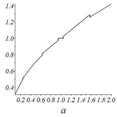
Discontinuities are related to different numbers of iterations of the Newton operator. 

> plot(g(a, 0.5e-1, 1.), a = .1 .. 2.000, font = [TIMES, ITALIC, 18], labelfont = [TIMES, ITALIC, 26])
 

Plot_2d
 

A "memory" version that start from the last computed value to save time. 

> g2 := proc (a, epsilon) local x, b; global p_res; if type(p_res, numeric) then x := p_res else x := 1 end if; if type(`+`(a, epsilon), numeric) then b := `/`(`*`(a), `*`(x)); while evalb(`<`(epsilon, ...
g2 := proc (a, epsilon) local x, b; global p_res; if type(p_res, numeric) then x := p_res else x := 1 end if; if type(`+`(a, epsilon), numeric) then b := `/`(`*`(a), `*`(x)); while evalb(`<`(epsilon, ...
 

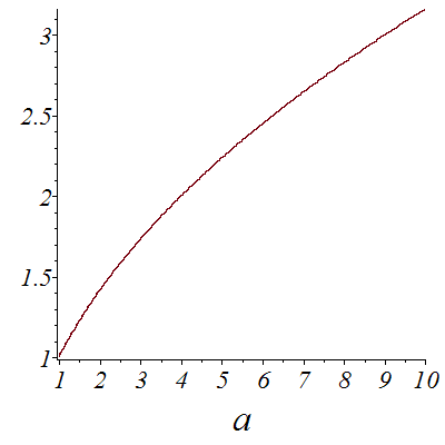
The curve looks smooth. 

> plot(g2(a, 0.1e-2), a = 1 .. 10, font = [TIMES, ITALIC, 18], labelfont = [TIMES, ITALIC, 26])
 

Plot_2d
 

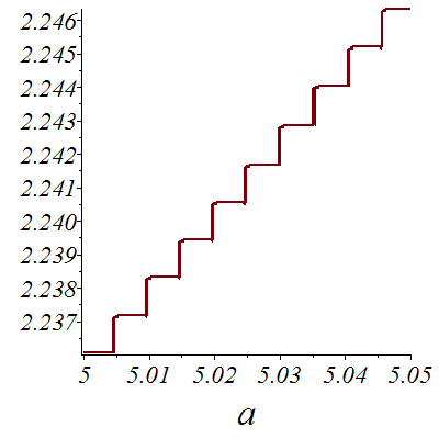
But is has many discontinuities and a derivative that is 0 where it is defined! 

> plot(g2(a, 0.1e-2), a = 5.0 .. 5.05, font = [TIMES, ITALIC, 18], labelfont = [TIMES, ITALIC, 26])
 

Plot_2d
 

Computing derivations with the "RootOf" Maple function, which is used when no closed form solution is found by "solve". 

> c := solve(`+`(`*`(`^`(x, 3)), exp(x)) = b, x); 1; solve(`*`(`^`(x, 2)) = b, x)


RootOf(`+`(exp(_Z), `*`(`^`(_Z, 3)), `-`(b)))
`*`(`^`(b, `/`(1, 2))), `+`(`-`(`*`(`^`(b, `/`(1, 2))))) (2)
 

The results are correct! 

> diff(c, b), diff(RootOf(`+`(`*`(`^`(_Z, 2)), `-`(b))), b)
 

`/`(1, `*`(`+`(exp(RootOf(`+`(exp(_Z), `*`(`^`(_Z, 3)), `-`(b)))), `*`(3, `*`(`^`(RootOf(`+`(exp(_Z), `*`(`^`(_Z, 3)), `-`(b))), 2)))))), `+`(`/`(`*`(`/`(1, 2)), `*`(RootOf(`+`(`*`(`^`(_Z, 2)), `-`(b)... (3)
 

Trying to look at Maple's internal definitions. 

> apply(eval(`diff/RootOf`), P(_Z, b), b)
 

`+`(`-`(`/`(`*`((D[2](P))(RootOf(P(_Z, b)), b)), `*`((D[1](P))(RootOf(P(_Z, b)), b))))) (4)
 

A "power series" version of our Newton operator, used to compute higher order derivatives. The global variable "nIter" keeps the number of iterations. 

> h := proc (a, eta, c, n, m) local x, b, d, epsilon; global nIter; nIter := 0; x := c; if type(`+`(a, eta, c, n, m), numeric) then b := `/`(`*`(`+`(a, epsilon)), `*`(x)); while evalb(`<`(eta, abs(subs(...
h := proc (a, eta, c, n, m) local x, b, d, epsilon; global nIter; nIter := 0; x := c; if type(`+`(a, eta, c, n, m), numeric) then b := `/`(`*`(`+`(a, epsilon)), `*`(x)); while evalb(`<`(eta, abs(subs(...
 

Computing the derivative of order 20. 

> h(2., 0.1e-3, 1., 20, 19), nIter
 

1141438794., 3 (5)
 

> subs(b = 2., diff(`*`(`^`(b, `/`(1, 2))), `$`(b, 19)))
 

1140326912. (6)
 

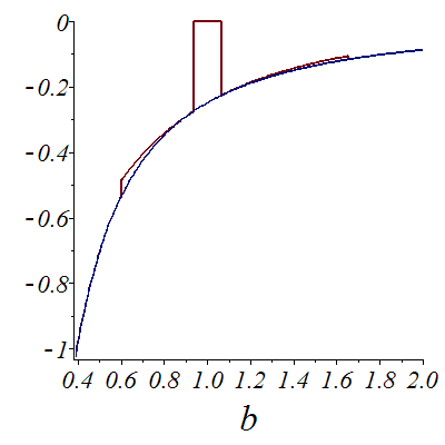
The derivative of the square root function computed with Newton compared with the actual values. The result is false near initial value 1. where no ieration is computed. 

> plot([h(b, 0.1e-2, 1., 10, 2), diff(`*`(`^`(b, `/`(1, 2))), `$`(b, 2))], b = .39 .. 2.00, axes = framed, font = [TIMES, ITALIC, 18], labelfont = [TIMES, ITALIC, 26])
plot([h(b, 0.1e-2, 1., 10, 2), diff(`*`(`^`(b, `/`(1, 2))), `$`(b, 2))], b = .39 .. 2.00, axes = framed, font = [TIMES, ITALIC, 18], labelfont = [TIMES, ITALIC, 26])
 

Plot_2d
 

>