By Alwen Tiu (tiu@cse.psu.edu, tiu@lix.polytechnique.fr )
Basic Linc (BLinc, pronounced 'blink') is an implementation of the sequent calculus of the logic Linc. Linc itself is an intuitionistic logic extended with explicit induction and co-induction rules. The logic was designed by Dale Miller (INRIA), Alberto Momigliano (LFCS, Edinburgh) and Alwen Tiu (student at Penn State University and currently visiting Ecole Polytechnique). The current version of the implementation was done by Alwen Tiu.
This tools is intended for expert users, and therefore basic knowledge in proof theory in general and the familiarity with the logic Linc are assumed. For a detailed description of the logic, users may want to consult [Tiu03]. Note that BLinc is not yet a theorem prover since it does not have the high-level tactical supports. The level of automation is still minimal. Nevertheless, it could be quite a useful tools for experimenting with proof search, e.g., it solves the representation issues (by employing higher-order abstract syntax), it has unification algorithm built-in, and, of course, it manages the task of substituting complex terms into another term, performs type checking etc. In short, if you are dealing with logical expressions too complex and cumbersome to manipulate manually on a sheet of paper, this tools should help you do all the uninteresting mechanics.
Basic Linc
Copyright (C) 2003 Alwen Tiu
This program is free software; you can redistribute it and/or modify it under
the terms of the GNU General Public License as published by the Free Software
Foundation; either version 2 of the License, or (at your option) any later
version.
This program is distributed in the hope that it will be useful, but WITHOUT ANY
WARRANTY; without even the implied warranty of MERCHANTABILITY or FITNESS FOR A
PARTICULAR PURPOSE. See the GNU General Public License for more details.
You should have received a copy of the GNU General Public License along with
this program; if not, write to the Free Software Foundation,
Inc., 59 Temple Place, Suite 330, Boston, MA 02111-1307 USA.
Some requirements to get BLinc started.
You must have the Sun Java runtime environment installed. The current version has been tested on Java version 1.4.2. The latest Java runtime environment can be found at http://java.sun.com.
You must have the Teyjus implementation of Lambda Prolog installed. The PATH environment must be set so that you can run 'tjsim' from a shell (in Unix) or a command prompt (Windows). The Teyjus distribution is available at http://teyjus.cs.umn.edu/ .
The following sections show how to use BLinc through a series of examples.
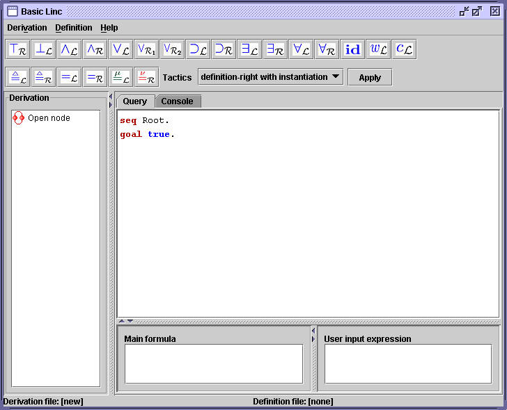
The interface for BLinc consists of three main panels. The top panel contains a toolbar consisting of the buttons corresponding to the inference rules of Linc. The left panel presents the derivation tree and the right panel contains detailed information about sequents, definitions and console (to be explained later).
Each derivation in Linc is parameterized upon a definition, which contains declaration of types and function/predicate symbols used in the derivation. This section shows how to create new definition and sequent and shows how to apply the inference rules.
To create a new definition file, choose the menu 'Definition' followed by 'New Definition'. The tab 'Definition' in the lowest panel will come into focus.
Figure 1. BLinc interface
Type in the following definition:
def test.
type p, q, r o.
ind
p <=> false.
ind
q <=> false.
ind r <=> false.
The statement 'def test.' declares the name of the definition. Note that each statement must be ended by a '.' (dot). The next statement declares that the symbol 'p', 'q' and 'r' are of type 'o'. The type 'o' is a built in type (the only one, for the moment) for denoting propositions. The last three statements are the definition clauses for the predicates p, q and r. The keyword 'ind' indicates that these are inductive definition. Note that each definition clause must be classified as either inductive (via the keyword 'ind') or coinductive (via 'coind'). The symbol 'false' is a built in logical constant, representing false, of course. Same for the symbol 'true'.
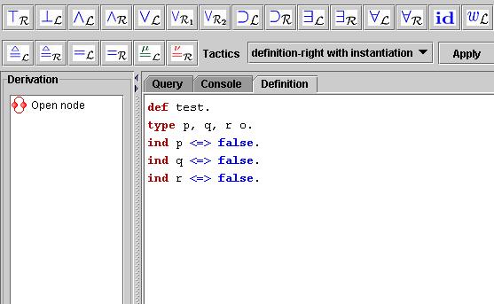
Figure 2. New definition
Now we are ready to prove some sequents. First we click on the node 'seq Root' in the left panel.
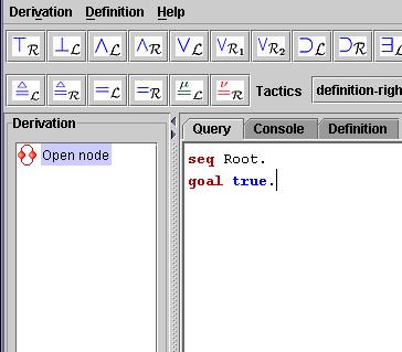
Figure 3. A simple sequent
This will switch us to the 'Query' tab in the right panel.
The symbol ![]() beside 'seq Root' indicates that
this sequent is still open, that is, no rule is applied to it yet.
beside 'seq Root' indicates that
this sequent is still open, that is, no rule is applied to it yet.
It will display the default sequent:
seq Root.
goal true.
A sequent consists of three parts: sequent's name (prefixed by the keyword 'seq'), hypothesis (prefixed by 'hyp') and goal (prefixed by 'goal'). The hypothesis part is optional. Again, as in the case with definition, each statement in a sequent must ends with a dot. Now let's change the above sequent to a more interesting one.
seq Root.
goal (p ; r) & (q ; r) => (p & q) ; r.
The symbol '&', ';' and '=>' represent the logical constants for
conjunction, disjunction and implication, respectively. The top most logical
constant in the formula is '=>', therefore we apply the implication-right rule.
This can be done by clicking on the button ![]() on
the toolbar. The resulting sequent is as follows.
on
the toolbar. The resulting sequent is as follows.
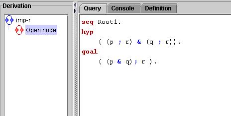
Figure 4. Applying implication-right rule
Notice that the label of the root node has changed to 'imp-r', indicating that the implication right rule was applied to the sequent in the node.
Let's see how we can apply a left-introduction rule. Let's apply
the and-left rule. To do so we just click on the button
![]() . The following dialog will appear to let us
choose the hypothesis to apply the rule with.
. The following dialog will appear to let us
choose the hypothesis to apply the rule with.
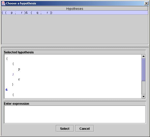
Figure 5. Applying and-left rule
The list on the top panel of the dialog presents available hypothesis with '&' as the main connective. The middle panel display the current selection of hypothesis. The lower panel is used to input terms, in case it is needed (e.g., in applying universal-left rule).
To see the description of the available rules in the toolbar,
just point to a particular button and wait until a tool tip appears. A successful application of
a rule may create new sequents
as a result. When no child sequents are produced, the node will be marked
as a leaf, indicated by the icon ![]() . An example of
a proof figure looks like this.
. An example of
a proof figure looks like this.
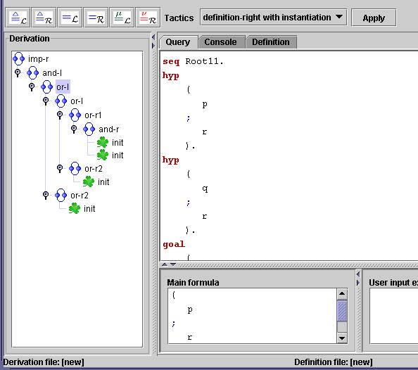
Figure 6. A proof figure
The derivation and the definition just created can be saved by selecting 'Save Derivation' and 'Save Definition' menu, respectively. The other menu items are pretty much self-explanatory. And there is the 'Console' tab which displays all the messages output by the server (the lambda Prolog program), if you are curious about what happens at the back end. Most of the time you won't need it. Any common errors will be reported through a friendly dialog box.
This section illustrates the use of higher-order terms (i.e., simply typed lambda terms), definition of base types and the use of induction. We won't show how to apply the co-induction rule since it is pretty much the same as how we use induction rule. We use the familiar append clause. If you are familiar with lambda Prolog you should have no difficulty reading the definitions.
The definition for the append clause is as follows.
def append.
kind list type.
kind int type.
type nil list.
type z int.
type s int -> int.
type conc int -> list -> list.
type app list -> list -> list -> o.
ind app <=>
l1:list\ l2:list\ l3:list\
(l1 = nil & l2 = l3) ;
(
sigma
l1':list\ sigma l3':list\sigma x:int\
l1 = (conc x
l1') & l3 = (conc x l3') & app l1' l2 l3'
).
% This is a comment and is ignored by parser.
The keyword 'kind' is used to declare a new base type. There is no support for introducing type constructors. The only type constructor available is the built-in arrow constructor '->'. Here we are declaring the type 'list' which is to denote list of integer. The type 'int' has the usual constructor 'z' (for zero) and 's' (for successor). The list constructors are 'conc' for building a list out of an integer and another list, and the constant 'nil' denoting the empty list. The symbol '=' denotes the built-in equality predicate. You can add comment lines by prefixing the line with the '%' symbol.
In defining 'app', we use a (unfortunately) more complicated syntax than the usual one in Prolog. That is, all pattern matching is encoded in the body of the definition clause. The head and the body of the definition clause is separated with '<=>'. The head is just the predicate symbol being defined, prefixed by the keyword 'ind' (or 'coind' if it's co-inductive definition). The arguments are abstracted using lambda abstractions. The keyword 'sigma' denotes existential quantification and 'pi' denotes the universal counterpart. The type of the body of the definition of 'app' must match the type of app, that is 'list -> list -> list -> o'.
We are interested in proving the judgment:
seq app.
goal pi l1:list\ pi l2:list\ app l1 l2 l1 => l2 = nil.
That is, if appending the two lists l1 and l2 results in l1, then l2 must be an empty list. We need to do two pi-right rules followed by the implication-right rule to get to the sequent
seq app111.
type E_1 list.
type E_0 list.
hyp
(app E_0 E_1 E_0).
goal
E_1 = nil.
There is a shorter way to get to the above sequent by using the 'focusing tactic'. This basically automates the introduction rules for all asynchronous connectives (explained in the section on focusing). To apply the focusing tactic, choose the entry 'focusing' in the 'Tactics' list in the toolbar and click the button 'Apply'. The variables E_0 and E_0 are fresh eigenvariables generated by the proof system.
We now apply the induction rule (by clicking the button
![]() in the toolbar). The 'Choose hypothesis'
dialog will appear, and we'll choose the (only) entry for the inductive
predicate in the hypothesis list. We must also type in the invariant in the textbox labelled
by 'Enter Expression'. We use the following invariant:
in the toolbar). The 'Choose hypothesis'
dialog will appear, and we'll choose the (only) entry for the inductive
predicate in the hypothesis list. We must also type in the invariant in the textbox labelled
by 'Enter Expression'. We use the following invariant:
l1:list\ l2:list\ l3:list\ (l1 = l3) => (l2 = nil)
The invariant must be of the same type as 'app'. The user interface at this stage will look like this (well, after some editing. The original computer-generated output contains more line breaks).
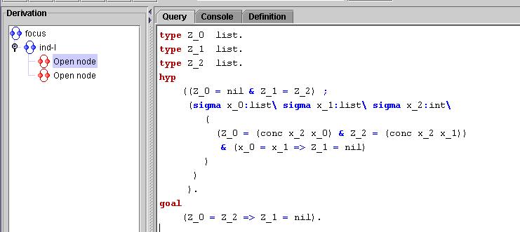
Figure 7. Applying induction
The sequent shown in the figure above is the 'inductive' part of the proof-search. That is, a proof of this sequent shows that the invariant we just put in is really a pre-fixed point of the corresponding definition of app.
Now at this stage I would suggest that you use the focusing tactic. It will save you 7 clicks at least. It will produce two sequents,
seq app1111111.
type Z_0 list.
type Z_1 list.
type Z_2 list.
hyp
Z_0 = nil.
hyp
Z_1 = Z_2.
hyp
Z_0 = Z_2.
goal
Z_1 = nil.
and
seq app11111211111.
type E_2 int.
type E_1 list.
type E_0 list.
type Z_0 list.
type Z_1 list.
type Z_2 list.
hyp
Z_0 = (conc E_2 E_0).
hyp
Z_2 = (conc E_2 E_1).
hyp
(E_0 = E_1 => Z_1 = nil).
hyp
Z_0 = Z_2.
goal
Z_1 = nil.
What remains are some simple equations which can be solved by using equality-left rule (unification).
The definition clauses might produce a big and complex formula if used in definition-right rule. Typically a definition clause will consists of a disjunction of several subformulas with equations and there is usually only one matching sub-clauses among the disjunctions. The problem is how to 'spot' the matching sub-clauses. For this purpose we introduce a tactic called 'definition-right instantiate' in the tactics selection list. When this rule is applied, it will try to list all the sub-clauses and give the user three options: to try all possible clause and instantiation (the button 'Try All'), to select a clause and try to instantiate (the button 'Instantiate'), or just select the clause without instantiating (the button 'Select'). The following figure illustrates an example using append clause defined in previous section.
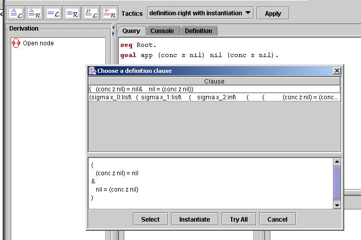
Figure 8. Instantiating definition-right
In a proof search of a sequent, certain introduction rules can be always applied be applied first without destroying provability of the sequent. The connectives corresponding to the introduction rules are called asynchronous connectives. Since we are using two sided sequent, we must differentiate between left-synchronous and right-synchronous. The left synchronous connectives are '&' (conjunction), ';' (disjunction) and 'sigma' (existential quantification). The right-synchronous ones are '&', '=>' and 'pi'. A derived rule, here called 'focusing', makes use of this fact, automates the application of these asynchronous connectives.
In fact, we can consider definition-left and equality-left as asynchronous rules as well. The combination of focusing with equality left has also been made available. However, since higher-order unification is undecidable in general, this tactic has to be used with caution.
Implement stratification checking on definition.
The implementation of induction and co-induction rules in current version assume that there is no mutual recursion. Will fix this in future release.
Improvements on the editor: syntax highlighting, more informative parser.
Rule applications: implement the 'prove-by-pointing' method, as it was used in PCoq interface for Coq, for example.
Tactical supports. Allow user to define high-level tactics. Need to build another parser for tactics file.
Re-implement the proof engine, probably in some other language, for better performance.
etc.. I'm sure there are plenty of them. Please let me know if you have suggestions or bugs to report.
[Tiu03] A logic for reasoning about logical specification. PhD thesis proposal. Penn State University, 2003. Available online at http://www.cse.psu.edu/~tiu/prop.pdf